3.1 Denotation of the variables and constants.
. . The author uses the variable X in program in stead of the independent variable t and denotes the range [t0, tmax] where the differential equation is solved by [XB, XE]. The range is divided in N equidistant intervals such that every interval is smaller than one. The interval is denoted by H0 and corresponds to the interval where the differential equation is solved by Runge-Kutta's method. Numbering the intervals from 1 to N and denoting an arbitrary number i by IB, the equidistant points ti=t0+H0×i are calculated by X=XB+H0*IB. The value IB denotes the end point of the interval and the point is denoted by X1 if the interval is not divided. The point denoted by the value IB−1 is denoted by X0. These calculated points are not equidistant by the error which is increased by the increase of IB. Supposing the range is [0, 13] and the N value is 300, the decimal system using five figures gives the following, when IB is 277.
 ____(3.1)
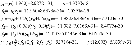
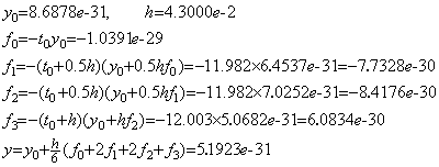
. . When the differential equation y' =−ty, y(0)=10 is solved by Runge-Kutta's method using the interval H0 in Eq. (3.1), the solution at X1 for IB=277 has no significant figure. In the case, if the exact solution is given in a five figure decimal as the initial value at X0, the solution at X1 is obtained, where the error is depend on the difference of the interval H0 and the valid interval H as follows.


. . The exact solution for comparison of accuracy must not be calculated at the equidistant points ti=t0+H0×i. It must be the exact solution at the points X=XB+H0*IB rounded in single precision because the differential equation is solved by use of the points X. The exact solution for i=277 is,


. . The author's method is similar and the method using three points denotes a half of the valid interval by H and the method using five points denotes one fourth of the valid interval by H. The three points are denoted by X0, X1, X2 and the five points are denoted by X0, X1, X2, X3, X4. The initial values y0, y0' , y0", ……… at X0 are denoted by the elements of array Y0(1), Y0(2), Y0(3), ……… respectively. The solutions y1, y1' , y1", ……… at X1 are denoted by the elements of array Y1(1), Y1(2), Y1(3), ……… respectively and so on.
. . The variable X denotes one of the variables X0, X1, X2, ……… and the elements of array Y(1), Y(2), Y(3), ……… denote the solution y and the derivatives y' , y", ……… at X respectively. These variables interface the subroutine given by user with the main program. The subroutine consists of three subroutines as,
| 56 F=-2*Y(1)-2*Y(2):RETURN 58 XB=0:XE=90:N=900:ND=2:Y(1)=0:Y(2)=1:RETURN 60 Y#=EXP(-X#)*SIN(X#):RETURN |
. . In case of the solution using the integral matrix, the elements of array Y1(1), Y1(2), Y1(3), ……… denote the differences Δy, Δy' , Δy", ……… respectively and the elements of array Y2(1), Y2(2), Y2(3), ……… denote the differences Δ2y, Δ2y' , Δ2y", ……… respectively. In case of the solution using the integral matrix of higher order than third order, these arrays are denoted by the array DY(j, k), where the elements of j≥1 and k≥1 denote the differences of derivatives Δ(k−1)y(j−1).
. . The solution using the variable interval divides the valid interval H0 in two equidistant intervals denoted by H1 and integrates every interval by the method using three points or five points, if the solution of the valid interval does not converge. The number of divisions is denoted by EE so the interval H1 is H1=H0/EE and the variable EB denotes the former half by the value 1 and the latter half by the value 2. If the solution of the former half does not converge, the both halves are divided in two equidistant intervals and the EE value becomes four. The variable EB has the values from one to four and the variable ES denotes the first interval, that is, ES=1. If the solution of the former half converges and the solution of the latter half does not converge, the latter half is divided in two equidistant intervals and the EE value becomes four, regarding the former half as divided. The variable ES is set the value 3 and the variable EB has the values 3 and 4, because the first and second interval have been solved already. If the solutions of all the divided intervals converge, next valid interval H0 is solved by use of EE=4. If the solution of any interval does not converge the EE value becomes eight. If the solution of the interval whose EB value is even satisfies the condition by which the divided two intervals may be merged into one interval, the EE value becomes a half of it.
3.2 Some algorithms for the operational calculus.
. .
The every element Δk+1y0 expressed in the integral operation ΔY=hD−1F must be calculated by Eq. (3.2) in order to avoid the increase of rounding error by summation.
 ____(3.2)
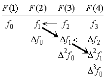
. . In order to transform the values of function f0, f1, f2, ……… into the successive differences Δf0, Δ2f0, Δ3f0, ………, the binomial expression should not be used, because it may cause a large amount of error by cancellation. The differences are calculated by use of the difference table as shown in Fig. 3.1. The F(4) value becomes Δf2 by subtracting F(3) from F(4) and the variables F(3) and F(4) become the elements of the vector F2=(f2, Δf2). Setting the variable F(2) as the first element, the two subtractions denoted by the arrows obtain the vector F1=(f1, Δf1, Δ2f1) when these are carried out by the order denoted by the bold arrows. Then, setting the variable F(1) as the first element, the three subtractions similar to above method obtain the vector F0=(f0, Δf0, Δ2f0, Δ3f0).
 | ________ |  |
| Fig. 3.1 | Fig. 3.2 |
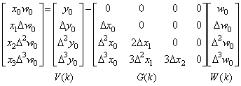
. . When the differential equation is y' =−ty, the function of the right side is the product of the function x(t)=−t and the function y(t). In case of the method using the vector calculus, the subroutine giving the function may be expressed in the product of the two vectors X and Y. The product must be carried out by expanding the vector X into the matrix. The matrix is obtained by multiplying the binomial coefficients to the matrix expressed in the difference table of Fig. 3.3 and the elements of the product are expressed in the expression of W(k). The equivalent results are obtained by use of the matrix expressed in the difference table of Fig. 3.3, if the summation is carried out by multiplying the binomial coefficients to the products of every element of a row of the matrix and the corresponding element of the vector Y. This calculation can be carried out without use of two dimensional array by varying the values of the array G(k) as shown by arrows.

Fig. 3.3
| [1] | . .The array G(k) is set the vector X and W(1) is obtained by G(1)×V(1). |
| [2] | . .Adding G(2) to G(1), G(1) becomes x1 and W(2) is obtained by G(2)×V(1)+G(1)×V(2). |
| [3] | . .Adding G(3) to G(2), G(2) becomes Δx1 and adding G(2) to G(1), G(1) becomes x2. Giving the array C(k) the products C(1)=G(3)×V(1), C(2)=G(2)×V(2), C(3)=G(1)×V(3), W(3) is obtained by the method shown in Fig. 3.2 as C(3)=C(1)+2C(2)+C(3). |
| [4] | . .Adding G(4) to G(3), adding G(3) to G(2), and adding G(2) to G(1), the array G(k) obtains the last row of the matrix of Fig. 3.3 and the array C(k) obtains G(5−k)×V(k). W(4) becomes C(4)=C(1)+3C(2)+3C(3)+C(4) by the method shown in Fig. 3.2. |
. . Program 3.1 is the subroutine carrying out above procedure. It is called by giving the array G(k) the multiplicand vector, giving the array V(k) the multiplier vector and giving the variable E2 the number of elements. It returns the array W(k) the product.
| Program 3.1__Vector W=G×V,__(E2=number of elements) |
|
50 FOR J7=1 TO E2:FOR J9=1 TO J7:J8=J7-J9+1 52 C(J9)=G(J8)*V(J9):GOSUB 56:NEXT J9:GOSUB 54:W(J7)=C(J7):NEXT J7:RETURN 54 IF J7>1 THEN FOR J9=2 TO J7:FOR J8=J7-J9+2 TO J7:C(J8)=C(J8)+C(J8-1): . .NEXT J8,J9:RETURN ELSE RETURN 56 IF J8>1 THEN G(J8-1)=G(J8-1)+G(J8):RETURN ELSE RETURN |
. . The quotient of vectors W=Y/X is calculated by post-multiplying the vector Y to the inverse matrix of the matrix X to which the vector X is expanded, that is, it is expressed in W=X−1Y. However, it may be calculated by changing the quotient into the product XW=Y and transposing the product of the matrix X and the vector W except of the diagonal elements to the right side as in Eq. (3.3). The product of the matrix and the vector W in Eq.(3.3) is carried out by the procedure mentioned in Fig 3.3.
 ____(3.3)
| [1] | __W(1) is obtained by the first row of Eq. (3.3) as w0=y0/x0. |
| [2] | __
Adding G(2) to G(1), G(1) becomes x1. Substituting 0×W(2)=0 for C(1) and G(2)×W(1)=Δx0×w0 for C(2), the summation shown in Fig. 3.2 obtains C(2)=Δx0×w0 and W(2) becomes {V(2)−C(2)}/G(1)={Δy0−Δx0×w0}/x1. |
| [3] | __
Adding G(3) to G(2), G(2) becomes Δx1 and adding G(2) to G(1), G(1) becomes x2. Substituting 0×W(3)=0 for C(1), G(2)×W(2)=Δx1×Δw0 for C(2) and G(3)×W(1)=Δ2x0×w0 for C(3), the summation shown in Fig. 3.2 obtains C(3)=C(1)+2C(2)+C(3) and W(3) is obtained by {V(3)−C(3)}/G(1). |
| [4] | __
Adding G(4) to G(3), G(3) becomes Δ2x1 and adding G(3) to G(2), G(2) becomes Δx2 and adding G(2) to G(1), G(1) becomes x3. Summating C(1)=0×W(4)=0, C(2)=G(2)×W(3), C(3)=G(3)×W(2) and C(4)=G(4)×W(1) by the method in Fig. 3.2, C(4) becomes C(1)+3C(2)+3C(3)+C(4) and W(4) obtained by {V(4)−C(4)}/G(1). |
| [5] | __ If the calculation of the k-th row obtains G(1)=0, that is, xk−1=0, W(k) is not calculated. |
. . By the procedure [5], W(k) holds the preset value if xk−1 is zero. The reason is that the quotient wk−1=yk−1/xk−1 is indefinite and that the quotient must be given as the initial value of differential equation. In usual, the array W(k) may be preset the dividend. The summation of the products of the values C(k) and binomial coefficients may carried out by the subroutine in the line 54 of Program 3.1. The row of the matrix, that is, the values of G(k) may be calculated by the subroutine in the line 56 of Program 3.1. Hence, the subroutine calculating the quotient is expressed in Program 3.2.
| Program 3.2__Vector W=V/G=G−1×V, (E2=number of elements) |
| 46 FOR J7=1 TO E2:C(J7)=0:FOR J9=1 TO J7-1:J8=J7-J9+1:C(J9)=G(J8)*W(J9): __GOSUB 56:NEXT J9:GOSUB 54:IF G(1)<>0 THEN W(J7)=(V(J7)-C(J7))/G(1) 48 NEXT J7:RETURN |
. . Program 3.3 obtains the square root of the function y(t) in Eq. (3.4) for example of use of the product and quotient of vectors. The square root of any function can be obtained by Newton-Raphson's method using the author's operational calculus as mentioned in Chapter 4 Section 1.6. The solution is obtained there by the expression in Taylor's expansion, starting the iterative calculation by the square root of the initial value. However, the starting value may be any vector. Program 3.3 starts the iterative calculation by a half of the vector Y, whose components are the successive differences of the values of function at the three point t=0, 1, 2 and are calculated by Line 14 using Line 36. Line 14 also calculates the true square root of the vector Y for comparison of accuracy. Line 16 iterates testing convergence of the calculation Xn+1=0.5×(Xn+Y/Xn) carried out by Line 22. The result of Program 3.3 is represented in Table 3.1.
 ________(3.4)
| Program 3.3 Newton-Raphson's method by the operational calculus. |
|---|
|
10 DIM X(11),Y(11),V(11),C(11),G(11),W(11),TR#(11):DEFINT E,J 12 DEF FNY#(T#)=T#*T#+SQR(2#)' ****y(t) 14 E2=3:H=1:FOR J0=1 TO E2:TR#(J0)=FNY#(H*(J0-1)):NEXT:GOSUB 36:PRINT"Vector Y __=":FOR J0=1 TO E2:Y(J0)=TR#(J0):Y#=Y(J0):GOSUB 32:X(J0)=Y(J0)*.5:V(J0)=Y(J0): __ TR#(J0)=SQR(FNY#(H*(J0-1))):NEXT:GOSUB 36:PRINT:PRINT"Vector X=.5*(X+Y/X)" 16 WHILE 2:CC=C(E2):GOSUB 22:FOR J0=1 TO E2:C(J0)=X(J0):NEXT:J7=E2:GOSUB 54: __ FOR J0=1 TO E2:Y#=X(J0):GOSUB 32:NEXT:PRINT:IF CC<>C(E2) THEN WEND 18 PRINT"True X=":FOR J0=1 TO E2:Y#=TR#(J0):GOSUB 34:NEXT:PRINT:PRINT"x(t)=": __ FOR J0=1 TO E2:C(J0)=X(J0):NEXT:J7=E2:GOSUB 54:GOSUB 30 20 PRINT"True x(t)=":FOR J0=1 TO E2:Y#=SQR(FNY#(H*(J0-1))):GOSUB 34:NEXT:PRINT: . .END 22 FOR J0=1 TO E2:G(J0)=X(J0):W(J0)=Y(J0):NEXT:GOSUB 46:FOR J0=1 TO E2: __X(J0)=(W(J0)+X(J0))*.5:NEXT:RETURN 30 FOR J0=1 TO E2:Y#=C(J0):GOSUB 32:NEXT:PRINT:RETURN 32 PRINT USING"##.#######^^^^ ";Y#;:RETURN 34 PRINT USING"##.########^^^^ ";Y#;:RETURN 36 FOR J9=2 TO E2:FOR J8=E2-J9+2 TO E2:TR#(J8)=TR#(J8)-TR#(J8-1):NEXT J8,J9: . .RETURN 46 Program 3.2 50 Program 3.1 |
| Table 3.1 The results of Newton-Raphson's method. | ||
|---|---|---|
| Vector Y= | ||
| 1.4142135 | 1.0000000 | 2.0000000 |
| Vector X=.5*(X+Y/X) | ||
| 1.3535534 1.1991844 1.1892487 1.1892071 |
2.5000000D-01 3.5536221D-01 3.6452556D-01 3.6456686D-01 |
5.0000000D-01 4.1708899D-01 4.0854657D-01 4.0850544D-01 |
| True X= | ||
| 1.18920712 | 3.64566859D-01 | __4.08505437D-01 |
| x(t)= | ||
| 1.1892071 | 1.5537740 | 2.3268464 |
| True x(t)= | ||
| 1.18920712 | 1.55377397 | 2.32684627 |