Chapter 4.. .Differential equations and applications.
1. Differential equations of the first order.
1.1 The method of solution by this operational calculus.
. .
The differential equations of the first order can generally be expressed in the following equation, where f(y) depends on the function exciting the differential equation but the expression is omitted.
 ________(1.1)
 ______(1.2)
 ______(1.3)
 ______(1.4)
 ______(1.5)
. . When the right side function f depends on the solution y(t), the integral operation in Eq. (1.4) has the following relation for any Y and Z.

 ______(1.7)
 ________(1.8)
 ________(1.9)
. . If the initial value y0 is zero and the value f(y0) also is zero and the function f(y) has not the variable t except of y(t), the iterative method gives the solution which is identical with zero. If there exists a solution which is not identical with zero, the first iterative procedure must slightly be modified to obtain the solution. If one of the above conditions is not satisfied, the solution being not identical with zero is obtained.


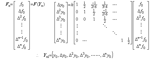
4)__In the same way, the correction with prediction is iterated until Yn−1 is obtained, where n is predetermined.


 ___(1.10)
. . If the norm of Yn1−Yn is less than the value ε, which is larger than the smallest value of the last significant decimal place of the numerical solution, the result Yn1 is the convergent solution. If the condition is not satisfied, there is the need to iterate the correction expressed in Eq. (1.10) once more by use of Yn1 instead of Yn. Denoting the result by Yn2, if the norm of Yn2−Yn1 is less than the value ε, the result Yn2 is the convergent solution. If the condition is not satisfied the result is not convergent yet. In the case, there is a need to increase the value n or to decrease the equidistant interval h if the condition (1.8) is not satisfied sufficiently or if the check is not made. In order to save the time spent on calculation, it is better to make the equidistant interval half.
. . In case of n=2 and n=4, the author showed the programs which does not use the vector calculus but transforms above vector equations into the expressions using the values yk, fk of the functions at equidistant points. However, it is better to use the vector calculus when the n value is larger than three, because the subroutine computing the product of the first row of the integral matrix and the operand vector can be used in order to compute all the products of the other rows and the operand vector. It makes the program simple and makes the parallel processing easy. The program and application are represented in Chapter 2 Section 5.
1.2 The solution by symbolical formula manipulation.
. .
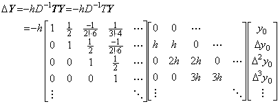
Denoting the equidistant interval by the symbol h, the elements of vectors are expressed in use of the symbol h. Using the integral matrix whose elements are the symbolical expressions in Eq. (1.10), the symbolical formula manipulation can obtain the solution expressed in the symbolical formula, which is Taylor's expansion with remainder, where the remainder has some errors.
. .
The differential equation y' =−ty, y(0)=1 has the solution expressed in Taylor's expansion with remainder as,
 ______(1.11)
. . Using the vectorial function, this differential equation is expressed in the vector equations as follows.
 _____(1.12)
 ____(1.13)
1)__

______The error is the remainder y' (ξ)h.

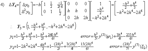
4)__Correcting Y3 by use of the integral matrix of order (3×4),
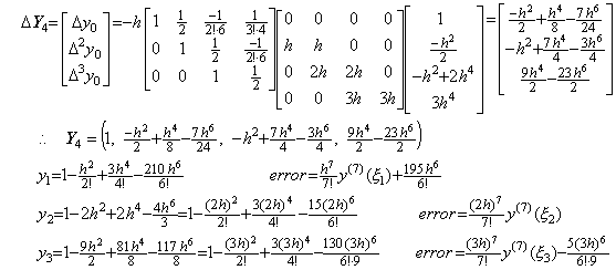
5)__Correcting Y4 by use of the integral matrix of order (3×4) once more,
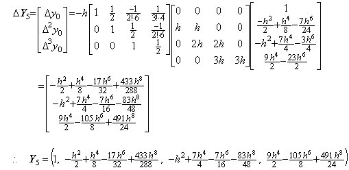

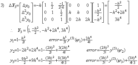
. . The solution expressed in the symbolical formula is the identical part between the results obtained by the twice correction. More than twice corrections using the integral matrix of order (3×4) do not yield the correct coefficient of the term with h6 and yield many terms which have h8, h9, ……… and whose coefficients are very large. These terms result in irregular numerical solution if the interval 3h does not sufficiently satisfy the condition by which Taylor's expansion converges.However, it must be taken care that all the terms that are different from the higher order terms of Taylor's expansion are not always errors in practically numerical solutions. In order that the numerical solution is exact value, the remainder term is required, adding to the terms that are the same as Taylor's expansion with h4 and lower order. These higher order terms may be a part of the remainder term, so these are not always numerical error. The examples are shown in the numerical examples of the extrapolation method in the section 1.4.
. . In the case of Taylor's expansion in Eq. (1.11), calculating the successive differences of y(t) at t=0, h, 2h, 3h, the following results are obtained and comparing each element of the vector solved above with the following results, the terms on and after h4 are not equal. However, the term h4 of the step 4) is equal to the term h4 of the step 5), so the term h4 is convergent. Furthermore, calculating the solutions y1, y2, y3 by use of the terms up to the term h4, these are equal to Taylor's expansion Eq. (1.11) up to the term h4. This shows that the term h4 need not be equal to Taylor's expansion and that it need be convergent. Accordingly, un-transforming the vector into the function, the deciding of convergence can be carried out by use of the elements of vector. In numerical solution too, it is able to use the same way.

. . In numerical calculation, the results of the step 3), 4) and 5) give the data by which it is able to decide whether the numerical solution converges or not. If there is no significant difference between the results of the step 3) and 4), the difference between the coefficients of the terms with h4 is not significant and the solution has been convergent. If there is some significant difference between them, the difference between the coefficients of the terms with h4 is significant. In the case, if there is no significant difference between the results of the step 4) and 5), the difference between the coefficients of the terms with h6 is not significant and the solution has been convergent. If there is some significant difference between them, the difference between the coefficients of the terms with h6 is significant and the solution is not convergent yet. In the case, if the interval 4h sufficiently satisfies the condition required by Taylor's expansion, the n value may be increased by one. If the interval 4h does not sufficiently satisfy the condition, the equidistant interval h must be decreased. These are the reason why the author's operational calculus uses the procedure mentioned in the preceding section.
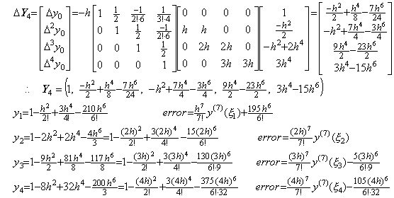
. . If the equidistant interval has been decreased the iterative method must be restarted from the step 1). If the n value has been increased it must be restarted from the step 1), or it must be continued from the step 4) by appending the fourth row of the integral matrix D−1. The result of the step 5) must not be used, because it has the terms which have h6 and h8 and whose coefficients are irregular. Accordingly, in case of n=4, the steps on and after 4) are modified as,
4)__Appending the fourth row of the integral matrix, Δ4y0 is appended to ΔY4 as,
5)__Correcting Y4 by use of the integral matrix of order (4×5),
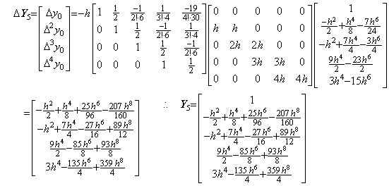
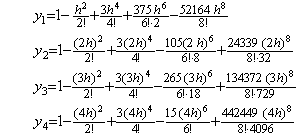
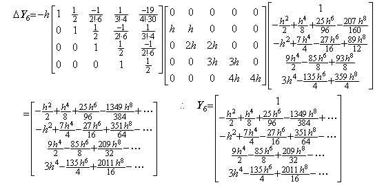
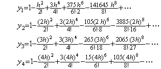
6)__Correcting Y5 by use of the integral matrix of order (4×5) once more,
. .
The predicting step 4) by use of the integral matrix of order four gives the result that only y2 has the correct terms up to h6. However, the correcting step 5) by use of the integral matrix of order (4×5) gives the result that only y4 has the correct terms up to h6. The step 6) correcting once more by use of the integral matrix of order (4×5) gives the result that all the terms up to h6 are convergent but the coefficients of the terms of h6 are not correct except y4 has the correct terms of h6 and h8. In order to obtain all the correct terms of h6, we must carried out the predicting step 5) by use of the integral matrix of order five and twice correcting steps by use of the integral matrix of order (5×6).
. .
These are the reason why the programs in Chapter 2 judge the convergence of the numerical solutions by the convergence of yn instead of the norm in case of using the integral matrix of order (n×(n+1)) and why they start to solve the next n intervals by use of yn as the initial value. The progress by one interval as usual predictor-corrector methods loses the accuracy and stability of the solution.
. .
Milne's predictor is of the same as the calculation of y4 in the above step 4) but its term of h6 is not correct. His corrector cannot make the term correct because it is Simpson's 1/3 rule, whose precision is worse than Milne's predictor. His predictor is obtained by use of the integral matrix of order four in step 5) of the preceding section as follows.
 _____(1.14)
 ___(1.15)
. . Substituting the values given by the differential equation into Milne's corrector and giving two accurate value y2, y3 expressed in Eq. (1.11) and the predicted value y4, where the error except of the term of h6 is denoted by ER,
 ____(1.16)
. . Usually Milne's method is regarded as the method integrating the interval h from t3=t0+3h to t4=t0+4h by use of the results y0, y1, y2, y3. However, it is the integral of the four intervals from t0 to t4 as shown in Eq. (1.15) and Eq. (1.16). In order to make the series convergent, it is required that the four intervals 4h sufficiently satisfy the condition which must make Taylor's expansion convergent. On the other hand, Runge-Kutta's method integrates the interval h by use of the half interval as shown below and requires that only the interval h must sufficiently satisfy the condition.

. . Table 1.1 shows the comparison of results in numerical calculation, where the initial value is y(0)=10. The column named Milne 1 shows the results of Milne's method using the corrector only once. The column named Milne 2 shows the results in case of using the corrector N times more as usual method, where the N values are shown in brackets and denote the convergence of solution except N=21 denotes no convergence. The one is more accurate and stable than the other after t=5. The iterative use of the corrector has almost no effect except of bud consequences after t=5.
. . The column named R.-K. 1 shows the results of Runge-Kutta's method integrating four intervals, which are the integral range of Milne's predictor. The results are slightly worse than Milne 1 and have no meaning after t=4. The column named R.-K. 2 shows the results of Runge-Kutta's method integrating two intervals, which are the integral range of Milne's corrector. The results are slightly better than Milne 1 around t=0 but they become worse than Milne 1 after t=1.6. The column named R.-K. 3 shows the results of Runge-Kutta's method integrating one interval, which is the integral range used by usual comparison of the two methods. The results are better than Milne 1 but the comparison has no meaning because the integral range is a half of Milne's corrector.
| Table 1.1 Comparison of Milne's method with Runge-Kutta's method. | |||||||
|---|---|---|---|---|---|---|---|
| t | Milne 1 | [N] Milne 2 | True | 10n | R.-K. 1 | R.-K. 2 | R.-K.3 |
| -0.2 -0.1 0.0 0.1 0.2 0.3 0.4 0.5 0.6 0.7 0.8 0.9 1.0 1.1 1.2 1.3 1.4 1.5 1.6 1.7 1.8 1.9 2.0 2.1 2.2 2.3 2.4 2.5 2.6 2.7 2.8 2.9 3.0 3.1 3.2 3.3 3.4 3.5 3.6 3.7 3.8 3.9 4.0 4.1 4.2 4.3 4.4 4.5 4.6 4.7 4.8 4.9 5.0 5.1 5.2 5.3 5.4 5.5 5.6 5.7 5.8 5.9 6.0 |
* * * * 9.801985 9.559971 9.231156 8.824958 8.352687 7.827025 7.261467 6.669740 6.065277 5.460712 4.867491 4.295543 3.753084 3.246501 2.780355 2.357447 1.978980 1.644742 1.353355 1.102511 8.892256 7.100641 5.613601 4.393810 3.404867 2.612241 1.984204 1.492146 1.110959 8.189017 5.976289 4.317867 3.088738 2.187330 1.533693 1.064518 7.316307 4.976955 3.352948 2.235188 1.476127 9.641744 6.242481 3.994103 2.535664 1.588600 9.891442 6.065259 3.704269 2.222832 1.330509 7.824053 4.573649 2.649826 1.498494 8.658934 4.659715 2.722967 1.388222 |
* * * * [1] 9.801985 [2] 9.559971 [2] 9.231157 [2] 8.824961 [2] 8.352690 [2] 7.827032 [2] 7.261475 [2] 6.669752 [2] 6.065289 [2] 5.460727 [21] 4.867506 [2] 4.295559 [2] 3.753097 [3] 3.246514 [2] 2.780364 [3] 2.357455 [3] 1.978982 [3] 1.644743 [3] 1.353352 [3] 1.102507 [4] 8.892171 [4] 7.100566 [3] 5.613492 [4] 4.393728 [3] 3.404758 [3] 2.612172 [4] 1.984113 [3] 1.492105 [3] 1.110893 [4] 8.188920 [21] 5.975855 [5] 4.318048 [5] 3.088463 [21] 2.187724 [5] 1.533482 [5] 1.065061 [5] 7.313908 [21] 4.983469 [4] 3.349478 [7] 2.242724 [6] 1.470929 [8] 9.730303 [7] 6.166814 [8] 4.102402 [8] 2.428532 [9] 1.726982 [8] 8.395819 [9] 7.900475 [9] 1.620723 [10] 4.726138 [10]-1.587930 [11] 4.269(-5) [21]-3.669(-5) [11] 5.203(-5) [11]-5.751(-5) [11] 7.179(-5) [11]-8.492(-5) [12] 1.035(-4) [21]-1.249(-4) |
9.80198673 9.95012479 1.00000000 9.95012479 9.80198673 9.55997478 9.23116344 8.82496903 8.35270199 7.82704545 7.26149030 6.66976789 6.06530660 5.46074412 4.86752228 4.29557318 3.75311111 3.24652467 2.78037290 2.35746057 1.97898674 1.64474464 1.35335283 1.10250492 8.89216081 7.10053615 5.61347500 4.39369336 3.40474421 2.61214065 1.98410974 1.49207819 1.11089965 8.18869738 5.97602198 4.31784069 3.08871441 2.18749112 1.53380989 1.06476605 7.31802551 4.97955236 3.35462628 2.23745881 1.47748183 9.65933345 6.25214775 4.00652974 2.54193577 1.59667624 9.92949522 6.11356511 3.72665317 2.24905706 1.34381028 7.94938558 4.65571332 2.69957850 1.54975396 8.80816483 4.95639984 2.76124090 1.52299797 |
+0 +0 +1 +0 +0 +0 +0 +0 +0 +0 +0 +0 +0 +0 +0 +0 +0 +0 +0 +0 +0 +0 +0 +0 -1 -1 -1 -1 -1 -1 -1 -1 -1 -2 -2 -2 -2 -2 -2 -2 -3 -3 -3 -3 -3 -4 -4 -4 -4 -4 -5 -5 -5 -5 -5 -6 -6 -6 -6 -7 -7 -7 -7 |
* * * * * * 9.231147 * * * 7.261394 * * * 4.867729 * * * 2.782125 * * * 1.357819 * * * 5.681144 * * * 2.055314 * * * 6.536229 * * * 1.879862 * * * 5.107530 * * * 1.390(-3) * * * 4.047(-4) * * * 1.345(-4) * * * 5.365(-5) * * * 2.659(-5) |
* * * * 9.801987 * 9.231163 * 8.352701 * 7.261490 * 6.065314 * 4.867548 * 3.753172 * 2.780485 * 1.979161 * 1.353590 * 8.895055 * 5.616689 * 3.408020 * 1.987196 * 1.113606 * 5.998208 * 3.105769 * 1.546143 * 7.402126 * 3.408833 * 1.510565 * 6.443620 * 2.647193 * 1.047986 * 4.000694 * 1.473920 * 5.245412 * 1.805212 * 6.015464 * 1.943720 |
* * * 9.950125 9.801987 9.559975 9.231163 8.824968 8.352701 7.827044 7.261489 6.669767 6.065306 5.460744 4.867524 4.295576 3.753114 3.246529 2.780379 2.357469 1.978997 1.644756 1.353366 1.102520 8.892320 7.100702 5.613648 4.393867 3.404918 2.612308 1.984269 1.492228 1.111037 8.189947 5.977133 4.318812 3.089554 2.188204 1.534407 1.065258 7.322023 4.982759 3.357159 2.239432 1.479001 9.670855 6.260771 4.012900 2.546580 1.600024 9.953292 6.130269 3.738234 2.256986 1.349177 7.985244 4.679385 2.715018 1.559705 8.871569 4.996307 2.786066 1.538262 |
. . In case of the integral of two intervals, the author's method gives following results expressed in symbolical formula by modifying the step 3) and 4) into correcting procedures using the integral matrix of order (2×3). The expression y2 of the step 4) is of the same as Runge-Kutta's result integrating two intervals 2h by use of the interval h as a half interval. Accordingly, the comparison of numerical results must be made with R.-K. 2.
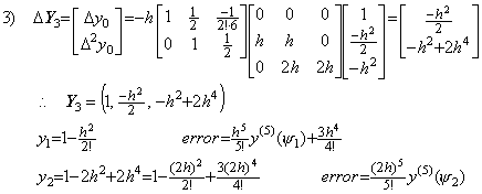
. . The program equivalent to this method is represented in Chapter 2 Section 1.3, where the vector calculus is not used. Rewriting the subroutines on and after the line 56 for solving above differential equation from zero to six by use of 30 equidistant intervals, it gives the result y=1.522434×10⁻⁷ at t=6. The result is better than R.-K. 3, which integrates a half of integral interval of the author's method. This shows that Runge-Kutta's method yields more errors in numerical calculation.
. . The author's method also is superior to usual methods by the reason that the results y2 of the step 2), 3) and 4) are the data by which we can determine the convergence of the solution y2 or the suitableness of integral interval and that we can obtain more accurate result by varying the integral interval. The author's variable interval method gives the result y=2.005017×10−36 at t=13.0 as shown in Table 2.7 of Chapter 2 Section 2.4. The true value of the solution is 2.00500878……×10−36.
1.3 Lipschitz condition.
. .
The value of integral operator is constant value, so the left side of Eq. (1.7) becomes,

 ____________(1.17)
Eq. (1.8) requires that there exists a constant k such that |F' (Y)|≤k is satisfied. Hence the vector-valued function
. . It is said that the differential equation in Eq. (1.18) cannot be solved by numerical calculus because the function f(y), that is, y' (y) does not satisfy Lipschitz condition as Eqs. (1.19).
 __________(1.18)
 ____(1.19)


 ______(1.20)
 ________(1.21)
. . The equation in Eq. (1.21) satisfies the condition Eq. (1.8) required in order to have the fixed point, independently of the h value. Supposing y>ξ>z>0,

. . The author's method is able to solve the differential equation by use of the fixed point in Eq. (1.20) as the integrand of the step 2), skipping the step 1).
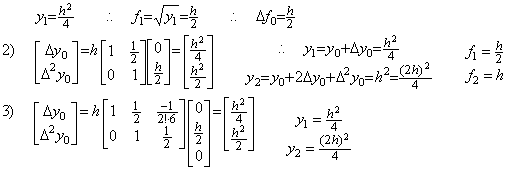
Usually, it is said that the solution of the differential equation in Eq. (1.18) is,
 for arbitrary c.______(1.22)
. . The above example is the case that the fixed point of the trapezoidal method is the accurate solution. Even if the fixed point is the approximate solution, the author's method is able to obtain the numerically correct result. In case of the differential equation in Eq. (1.12), the fixed point of the trapezoidal method is expressed in the series whose terms on and after h4 are not correct.


The result y2 is of the same as the result of the step 4) in the last of the previous section, if the terms on and after h8 are negligible numerically.
. . The numerical methods cannot solve the differential equation in Eq. (1.23), because the value f(0) is infinity. The reason is independent of Lipschitz condition because there exists the mean value f ' (ξ) as shown in Eq. (1.24), if yz≠0.
 ________(1.23)
 _____(1.24)
. . The trapezoidal method also is able to solve the differential equation if the initial value y0 is given at t=h when h is the equidistant interval. Supposing the value y1 is an arbitrary value at t=2h and iterating the trapezoidal method in Eq. (1.25), the solutions are given as shown in column A of Table 1.2, when the equidistant interval is h=0.1.
 ______(1.25)
| Table 1.2__y0=y(0.1), h=0.1 | |||
|---|---|---|---|
| t | A | B | True value |
| 0.1 0.2 0.3 0.4 0.5 : 1.0 2.0 3.0 4.0 5.0 : : 10.0 : : 100.0 |
0.447213 0.637454 0.779994 0.899673 1.00500 : 1.41819 2.00297 2.45196 2.83058 3.16421 : : 4.47352 : : 14.1426 |
0.450000 0.639319 0.781506 0.900981 1.00617 : 1.41902 2.00355 2.45243 2.83100 3.16459 : : 4.47378 : : 14.1427 |
(Initial value) 0.6324555 0.7745966 0.8944271 1.0000000 : 1.4142135 2.0000000 2.4494897 2.8284271 3.1622776 : : 4.4721359 : : 14.142135 |
These are equivalent to the fixed points of the following equations as to yk.
 _____(1.26)
. . The mean value of f0 and f1 of Eq. (1.25) is very different from the mean value of integral around t=0.1. The exact mean value f is given by the reciprocal of f0 and f1 as follows. Changing the independent variable into y by the reciprocal of the both sides of the differential equation in Eq. (1.23),

 __________(1.27)
| 0.4472136, 0.6708204, 0.6260990, 0.6335526, 0.6322675, 0.6324878, 0.6324500 0.6324565, 0.6324554, 0.6324556, 0.6324555 |

 ________(1.28)
| 1) | We obtain the solution t=δ at y=ε, which is very small. |
| 2) | Changing the independent variable into t, we obtain the solution y1 by the integral from t=δ to t=h of f(y). |
| 3) | We obtain the solution yk at t=kh, (k>1) with the initial value y1 at t=h. |
. . In case of the differential equation in Eq. (1.23), supposing ε is 0.1, the half interval is y=0.05 and the step 1) gives,

| 56 F=1/Y(1):RETURN 58 XB=0.005:XE=0.1:N=1:ND=1:Y(1)=0.1:EE=16:RETURN 60 Y#=SQR(X#):PRINT USING"True=##.########^^^^";Y#:RETURN |
. . The step 3) gives the solutions yk+1 at t=0.1+kh for k=IB as in Table 1.4, where Line 58 is,
| Table 1.3__The solution from t=0.005 to 0.1. | ||||
|---|---|---|---|---|
| EB | EE | t (10n) | y (10n) | True (10n) |
| 1 2 3 4 5 6 7 8 9 10 6 7 8 9 10 6 7 8 9 10 11 12 7 8 |
64 64 64 64 64 64 64 64 64 64 32 32 32 32 32 16 16 16 16 16 16 16 8 8 |
6.48438(-3) 7.96875(-3) 9.45313(-3) 0.0109375 0.0124219 0.0139062 0.0153906 0.016875 0.0183594 0.0198437 0.0228125 0.0257813 0.02875 0.0317187 0.0346875 0.040625 0.0465625 0.0525 0.0584375 0.064375 0.0703125 0.07625 0.088125 0.1 |
1.138805(-1) 1.262439(-1) 1.375001(-1) 1.479020(-1) 1.576190(-1) 1.667709(-1) 1.754459(-1) 1.837118(-1) 1.916214(-1) 1.992173(-1) 2.136001(-1) 2.270738(-1) 2.397916(-1) 2.518681(-1) 2.633914(-1) 2.850439(-1) 3.051640(-1) 3.240371(-1) 3.418699(-1) 3.588176(-1) 3.750001(-1) 3.905126(-1) 4.198215(-1) 4.472137(-1) |
1.13880419(-1) 1.26243811(-1) 1.37500002(-1) 1.47901993(-1) 1.57619004(-1) 1.66770799(-1) 1.75445862(-1) 1.83711734(-1) 1.91621377(-1) 1.99217217(-1) 2.13600096(-1) 2.27073783(-1) 2.39791578(-1) 2.51868019(-1) 2.63391346(-1) 2.85043851(-1) 3.05163891(-1) 3.24037030(-1) 3.41869859(-1) 3.58817497(-1) 3.75000000(-1) 3.90512488(-1) 4.19821403(-1) 4.47213599(-1) |
| Table 1.4__The solution from t=0.1 to 10. | |||||
|---|---|---|---|---|---|
| IB | EB | EE | t | y (10n) | True (10n) |
| 1 | 1 2 3 4 5 6 4 |
8 8 8 8 8 8 4 |
0.1125 0.125 0.1375 0.15 0.1625 0.175 0.2 |
4.743421(-1) 5.000004(-1) 5.244048(-1) 5.477229(-1) 5.700880(-1) 5.916082(-1) 6.324558(-1) |
4.74341658(-1) 5.00000000(-1) 5.24404430(-1) 5.47722568(-1) 5.70087702(-1) 5.91607973(-1) 6.32455537(-1) |
| 2 | 1 2 3 4 |
4 4 4 4 |
0.225 0.25 0.275 0.3 |
6.708207(-1) 7.071070(-1) 7.416201(-1) 7.745969(-1) |
6.70820407(-1) 7.07106781(-1) 7.41619857(-1) 7.74596646(-1) |
| 3 | 1 2 2 |
4 4 2 |
0.325 0.35 0.4 |
8.062260(-1) 8.366602(-1) 8.944274(-1) |
8.06225760(-1) 8.36660019(-1) 8.94427164(-1) |
| 4 | 1 2 |
2 2 |
0.45 0.5 |
9.486835(-1) 1.000000 |
9.48683285(-1) 9.99999970(-1) |
| 5 | 1 2 |
2 2 |
0.55 0.6 |
1.048809 1.095445 |
1.04880880 1.09544508 |
| 6 | 1 2 |
2 2 |
0.65 0.7 |
1.140176 1.183216 |
1.14017540 1.18321595 |
| 7 8 9 19 29 39 49 59 69 79 89 99 |
1 1 1 1 1 1 1 1 1 1 1 1 |
1 1 1 1 1 1 1 1 1 1 1 1 |
0.8 0.9 1 2 3 4 5 6 7 8 9 10 |
1.264911 1.341641 1.414214 2.000000 2.449490 2.828427 3.162278 3.464102 3.741658 4.000001 4.242641 4.472137 |
1.26491107 1.34164077 1.41421356 1.99999994 2.44948965 2.82842704 3.16227751 3.46410148 3.74165726 3.99999988 4.24264069 4.47213595 |
1.4 The solution by interpolation and extrapolation.
. .
The author's methods using the integral matrix of order n require n+1 equidistant points. Usually, these points are obtained by dividing the each integral interval by n as mentioned in previous section, when the integral interval is given by dividing the given integral range by the number of points at which the solutions should be obtained. Hence the author names them the solution by interpolation. It is similar to Runge-Kutta's method, which uses the predicted result at the half point of the integral interval except the way of using the result is different from the author's method using 3 points.
. .
The solution by interpolation is able to solve the differential equation by use of the variable interval into which every interval subdivided and by use of the integral matrix of variable order. However, it cannot integrate tabulated functions because it cannot obtain the values at equidistant points dividing the tabulated interval by n. In this case, the author's methods must use n tabulated interval to obtain the required n+1 equidistant points. The author names these the solution by extrapolation because these use the points t=t0+kh for k>1 in order to correct the solution at t=t0+h.
. .
The solution by extrapolation is able to use the integral matrix of a fixed order or variable order. The both methods are able to use two ways advancing the lower limit of integral. One advances to t0+nh if the integral matrix is of the order
. .
Table 1.5 shows the solution of the differential equation y' =−ty, y(0)=10 by the extrapolation using the equidistant interval h=0.1 and the integral matrix of variable order n≤11. The column IB is the equidistant points and the column E is the order of the integral matrix, that is, the corrector is of order ((E−1)×E). When IB is one, the solution at t=0.1 converges by use of the four equidistant points t=0, 0.1, 0.2, 0.3 and the solutions at t=0.2, 0.3 are not convergent, so the IB value is increased by 1. When IB is two, all the solutions converge at t=0.2, 0.3, 0.4, 0.5 by use of the solution at t=0.1 as the initial value, so the IB value is increased by four. When IB is equal to or larger than 28, the solution converges only at the point denoted by the IB value. When IB is equal to or larger than 52, the order of the integral matrix does not vary by the restriction given. The restriction loses the accuracy of solution. However, the loss is very slight, compared with Milne's method and Runge-Kutta's method shown in Table 1.1.
| Table 1.5 . .The solution by extrapolation of y' =−ty, y(0)=10. | ||||||||||
|---|---|---|---|---|---|---|---|---|---|---|
| IB | E | t | y (10n) | True (10n) | . . | IB | E | t | y (10n) | True (10n) |
| 1 2 6 7 10 14 15 16 21 22 28 29 30 31 32 33 34 |
4 5 4 4 5 6 6 6 6 7 7 7 8 6 6 7 7 |
0.1 0.2 0.3 0.4 0.5 0.6 0.7 0.8 0.9 1.0 1.1 1.2 1.3 1.4 1.5 1.6 1.7 1.8 1.9 2.0 2.1 2.2 2.3 2.4 2.5 2.6 2.7 2.8 2.9 3.0 3.1 3.2 3.3 3.4 |
9.950120(0) 9.801984(0) 9.559971(0) 9.231160(0) 8.824965(0) 8.352683(0) 7.827014(0) 7.261469(0) 6.669735(0) 6.065274(0) 5.460716(0) 4.867497(0) 4.295553(0) 3.753093(0) 3.246508(0) 2.780359(0) 2.357449(0) 1.978977(0) 1.644736(0) 1.353346(0) 1.102500(0) 8.892118(-1) 7.100501(-1) 5.613449(-1) 4.393672(-1) 3.404729(-1) 2.612128(-1) 1.984100(-1) 1.492071(-1) 1.110894(-1) 8.188665(-2) 5.975999(-2) 4.317823(-2) 3.088704(-2) |
9.95012479(0) 9.80198673(0) 9.55997478(0) 9.23116344(0) 8.82496903(0) 8.35270199(0) 7.82704545(0) 7.26149030(0) 6.66976789(0) 6.06530660(0) 5.46074412(0) 4.86752228(0) 4.29557318(0) 3.75311111(0) 3.24652467(0) 2.78037290(0) 2.35746057(0) 1.97898674(0) 1.64474464(0) 1.35335283(0) 1.10250492(0) 8.89216081(-1) 7.10053615(-1) 5.61347500(-1) 4.39369336(-1) 3.40474421(-1) 2.61214065(-1) 1.98410974(-1) 1.49207819(-1) 1.11089965(-1) 8.18869738(-2) 5.97602198(-2) 4.31784069(-2) 3.08871441(-2) |
35 : : : : 51 52 53 54 55 56 57 58 59 60 61 : : 89 90 91 |
7 : : : : 10 11 11 11 11 11 11 11 11 11 11 : : 10 11 11 |
3.5 : : : : 5.1 5.2 5.3 5.4 5.5 5.6 5.7 5.8 5.9 6.0 6.1 : : 8.9 9.0 9.1 9.2 9.3 9.4 9.5 9.6 9.7 9.8 9.9 10. |
2.187483(-02) : : : : 2.249050(-05) 1.343809(-05) 7.949373(-06) 4.655704(-06) 2.699572(-06) 1.549749(-06) 8.808157(-07) 4.956393(-07) 2.761235(-07) 1.522994(-07) 8.316679(-08) : : 6.306696(-17) 2.576850(-17) 1.042381(-17) 4.175947(-18) 1.660551(-18) 6.670604(-19) 3.025806(-19) 2.349915(-19) 4.096942(-19) 1.019628(-18) 2.731899(-18) 7.452993(-18) |
2.18749112(-02) : : : : 2.24905706(-05) 1.34381028(-05) 7.94938558(-06) 4.65571332(-06) 2.69957850(-06) 1.54975396(-06) 8.80816483(-07) 4.95639984(-07) 2.76124090(-07) 1.52299797(-07) 8.31670729(-08) : : 6.30615778(-17) 2.57675711(-17) 1.04240256(-17) 4.17501738(-18) 1.65551973(-18) 6.49931301(-19) 2.52616378(-19) 9.72094942(-20) 3.70353883(-20) 1.39694133(-20) 5.21670711(-21) 1.92874985(-21) | |
. . When IB is 91, the solutions are regarded as being convergent at all the points after t=9.1, because there are not eleven equidistant points in the range 9.1≤t≤10 if IB is increased to 92. The solutions after t=9.5 are very different from the exact solutions but these are useful to make the solution convergent at t=9.1. The case occurs always when the IB value is increased only by one as shown in Table 1.6. When the solution is convergent at t=5.2, the solutions after t=5.2 are not convergent and the solution at t=6 is as inaccurate as the result in R.-K. 3 of Table 1.1. It is said that by this reason Milne's method uses the predictor introduced by the backward interpolation formula and that it is able to predict the solution accurately at the last point. However, the idea is a mistake because Milne's predictor is of the same as Eq. (1.14) introduced by the forward interpolation formula. It is also said that the predictor-corrector methods using the polynomial of higher order are unstable. However, the cause is that the methods predict and correct the solution at the last point.
| Table 1.6 . .From 0 to 6 by h=0.1. | ||||
|---|---|---|---|---|
| IB | E | t | y (10−n) | True (10−n) |
: 46 47 48 49 50 51 52 |
: 9 9 10 10 10 10 10 |
: 4.6 4.7 4.8 4.9 5.0 5.1 5.2 5.3 5.4 5.5 5.6 5.7 5.8 5.9 6.0 |
: 2.541928(-4) 1.596674(-4) 9.929478(-5) 6.113552(-5) 3.726643(-5) 2.249050(-5) 1.343809(-5) 7.949374(-6) 4.655708(-6) 2.699582(-6) 1.549770(-6) 8.808545(-7) 4.957133(-7) 2.762749(-7) 1.526310(-7) |
: 2.54193577(-4) 1.59667624(-4) 9.92949522(-5) 6.11356511(-5) 3.72665317(-5) 2.24905706(-5) 1.34381028(-5) 7.94938558(-5) 4.65571332(-6) 2.69957850(-6) 1.54975396(-6) 8.80816483(-7) 4.95639984(-7) 2.76124090(-7) 1.52299797(-7) |
. . The numerical methods to solve the differential equations with ill condition must satisfy the following conditions. If they are of using the solution by interpolation, the equidistant interval must be variable and the integral matrix may be of variable order or fixed order. They must decide at the last point whether the solution is convergent or not. If they are of using the solution by extrapolation, the integral matrix is of variable order. They must decide at the next point of the initial value whether the solution is convergent or not. If the solutions are convergent at the successive k points, the next step may advance the initial point to the k-th point.
1.5 Taylor's expansion of a vectorial function.
. .
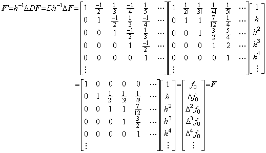
In order to solve the differential equation by the author's operational calculus using vector computer, the vector-valued function F(Y) of the differential equation y' =f(y) must be calculated by use of the vector Y immediately. In case of the usual computer, the vector values may be obtained by calculating the successive differences of the values fk for the solutions yk transformed from the vector Y at equidistant points. In the case, if the calculation causes the successive differences the cancellation of many significant figures, the solution may not get sufficient accuracy. In order to avoid it, the vector-valued function should be calculated by use of the vector Y immediately. Accordingly, the function F(Y) must be the vectorial function mentioned in Section 1.2. If the function is an irrational function it is calculated by use of Taylor's expansion usually.
. .
Carrying out Taylor's expansion of the function f(t) at every equidistant point tk=t0+kh for k≥0, and calculating the difference of the initial value f(tk) from the value f(tk+h) at t=tk+h of the every Taylor's expansion,
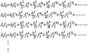
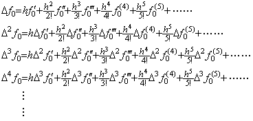
. .
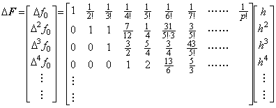
[Theorem 401]. .When f(t)∈Cp+1[a, b], Taylor's expansion of the vector ΔF which denotes the function Δf(t) is expressed in,
 _____(1.30)

. .
Accordingly, if the function f(y) is an irrational function of y, the differential equation Y' =F is equivalent to the differential equation of the (p+1)th order by substituting it into F of Eq. (1.30). However, if the successive derivatives of
 . .(1.31)
 ____(1.32)
. . When the vector T0 denotes the function t(u) and the vector T denotes the function t(u)+h, the vector T consists of the successive differences of t0+h, t1+h, t2+h, ………, tm+h. Hence,

. . When the vector T denotes the function t(u) from u0 to um and the vector T0 denotes the constant function t=t(u0)=t0,

 ____(1.33)
. . When the function t(u) is the function such that t(u)=t0+hu, the value of t(u) for the equidistant points u=0, 1, 2, 3, ……… are also equidistant and the function t(u) is expressed in the vector T=(t0, h, 0, 0, ………). Hence,
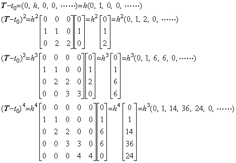
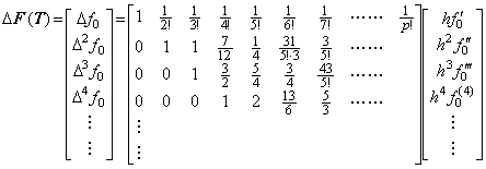 __(1.34)
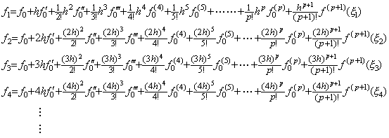
 ___(1.35)
where, _____n, m=1, 2, 3, 4, ……….
. .
[Theorem 402]. .In case of m≥n+1,
 ______(1.36)
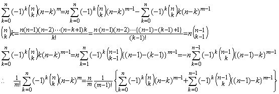
| [Q.E.D.] |
. . In case of the differential equation in Eq. (1.31), all the values f0", f0(3), f0(4), ……… are zero, so the matrix equation Eq. (1.34) becomes,

. . In general, if the differential equation is differentiable, the initial values y0(k) for the successive integer k can be obtained and the solution y(t) can be obtained by Taylor's expansion without integration. The numerical solutions can also be obtained by the matrix equation in Eq. (1.34), where the denotation F and f must be replaced with Y and y respectively. Accordingly, it is equivalent to the convergence of Taylor's expansion that there exists the numerical solution of the differential equation.
. . When we solve the differential equation of the first order expressed in y' =f(y) by use of the iterative integration, if the function f(y) is irrational, it may be expressed in Taylor's expansion which is the function of the independent variable y. The vectorial function F(Y) is expressed in Eq. (1.37) by replacing the denotation T and t of Eq. (1.33) with Y and y respectively.
 ____(1.37)

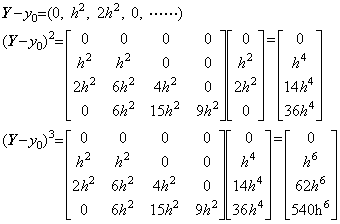
. . When the functions y(t) and f(y) are,
 ______(1.38)
 __(1.39)
 ____(1.40)
1.6 Newton-Raphson's method.
. .
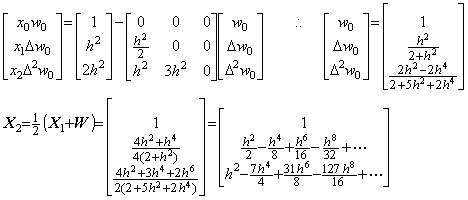
Denoting the square root of a number y by x, it is given by the point at which the locus of the function f(x)=x2−y intersects the x-axis. In the same way, denoting the square root of a vector Y by the vector X, it is given by the point at which the locus of the vectorial function F(X)=X2−Y intersects the X-axis on the plane denoting all the ordered pairs of vectors (X, F). The point is obtained by Newton-Raphson's method.
 _____(1.41)
 ___(1.42)
 ____(1.43)
1.7 The formulas for differentiation and integration.
. .
The author's differential and integral operators may be used as the symbolical operators to solve the differential equations. In the case, it must be cautioned that the multiplication of the operators and vectors does not always hold the same commutative and associative laws as the multiplication of numbers as mentioned in Chapter 2 Section 2.2. The differential equation in Eq. (1.18) of Section 1.3 may be solved by no use of the square root of the function y, squaring the both sides.
 ________(1.44)

. .
[Theorem 403]
 ________(1.45)


 ____[Q.E.D.]


 ____(1.46)
 ________(1.47)
. . The indefinite integral does not mean that there are many solutions of the differential equation but that the initial value is unknown. Hence the integral operation is unique. It is said that the differential operation obtains the one derivative g' (t) from all the functions with any constant c, that is, g(t)+c. However, the author says that the differential operation obtains the pair of the initial value and the derivative, that is, (g(0), g' (t)) and that the two operations are reversible.
. .
[Theorem 404]
 ______(1.48)
. .
[Theorem 405]
 ________(1.49)
. .
The differential equation y' =y−1, y(t0)=y0 may be solved by Theorem 405 as follows.


. .
[Theorem 406]. .When Y=eT, the derivative is Y' =eT.
[Proof]. .It is evident by y=et and y' =et.__________[Q.E.D.]
. .
The vectorial function eT is expressed in Taylor's expansion as,
 ________(1.50)
 ____(1.51)